How to Estimate Click-through Rate
If your work involves the display ads business, sooner or later you will need to analyze the click-through-rate data. This is a very typical metric used to capture the effectiveness of online advertising campaign. The Click-through Rate, or CTR, by definition, is the number of times a click is made on the advertisement (Click-throughs) divided by the the number of times an advertisement is displayed (Impressions):
Click-through rate = Click-through # / Impression #
If you want to compute the CTR for one piece of advertisement, the computation follows from the above formula, and you can stop reading now. However, since my title of this post is “how to ESTIMATE CTR”, and there is no point to talk about ESTIMATION in statistics unless you have a sample, the real problem that I am talking about is:
Suppose you get Click-throughs and impressions data for a number of campaigns, how to estimate the average CTR?
This may sound like a simple enough problem, but if you really have done such analysis you must have been overwhelmed by the real life complexities, most of them coming from design and sampling issues. A short post like this will not address all these problems and offer you a panacea. What it is able to do is to suggest a few simple, exploratory analyses that you may want to try.
Preparation
As usual, let’s first simulate a synthetic data set in R:
impressions <- as.integer(exp(rnorm(100, mean = 5, sd = 1)))
clicks <- rpois(100, lambda = 0.01 * impressions)
You may wonder why I select such weird distributions to simulate the data. This is to make the data look more like in reality, and to introduce some data transformation methods. But first, lets look at the simplest statistic:
Estimate the Mean CTR
This is straightforward:
meanCTR <- mean(clicks / impressions)
But again, if you take this number to your manager, an almost sure subsequent question is: what is the accuracy of your estimate? Do not groan on your manager’s fastidium: in statistics, estimation makes little sense without justifying its variability. So a side question that accompanies is: how to estimate the variance of your estimate?
Estimate the variance of your mean CTR estimate
This is a little tricky because the mean CTR is an average number of a sequence of ratios, and there is no off-the-shelf formula you can use to compute the variance of the mean ratio estimates. So what you can do?
Well, think the problem this way: what does the variance of your estimate tell you? It tells you the variability of your mean CTR estimate. How to describe the variability here? Suppose your data, which has 100 campaigns, is sampled from a huge number of campaigns, say 1 million. The variability means that, if you draw another sample of 100 campaigns from the 1 million campaign, and compute the mean CTR, how much difference is that from your current mean CTR? Now the problem is much simpler: if you have those 1 million data, you may just draw repetitively samples of 100 campaigns and compute the mean CTRs from these samples, and see what is the variance of these mean CTRs.
The only issue here is that you don’t have those 1 million data. In fact, you shouldn’t have, otherwise you should use those 1 million data instead of the sample of 100. So what to do? Well, you can make a naive assumption here: those 1 million data are just duplicating your sample 10,000 times. Now you can draw samples from them. Simple enough!
Actually this is the idea of bootstrap, which is very popular to deal with problems like this: estimate the variance where you do not have a formula off-the-shelf. And in implementing bootstrap you do not actually need to replace your sample 10,000, times; you just need to draw samples from your sample with replacement.
A chunk of codes for our synthetic data is the following:
bootstrapMCTR <- function(x) {
  set.seed(x)
  id <- sample(seq_along(clicks), 100, replace = TRUE)
  return(mean(clicks[id] / impressions[id]))
}
mCTRs <- sapply(seq(1000), bootstrapMCTR)
var(mCTRs)
Add weights to the campaigns
Different campaigns may be of different importance to you, so you may want to add some weights to reflect their importance. Suppose here we take the logarithm of the impressions as the weights. The estimate for mean CTR is:
my_weights <- log(impressions)
weightedMCTR <- mean(clicks / impressions, weights = my_weights)
For computing the variance, again use the bootstrap method. It is a bit tricky to use the weights here: you should use weights as the sampling probabilities, and DO NOT use weights in computing the bootstrapped sample mean CTRs. You can reason it through the imaginary 1 million data sets. In constructing such data, rather than replace each campaign 10,000 times, the number of duplications for each campaign should be proportional to its weight. Drawing non-weighted random samples from this data is just like drawing weighted samples from the original data. Because this 1 million data already have more duplicates for campaigns with higher weights, you no longer need to adjust their weights in the sample mean.
weightedBootstrapMCTR <- function(x) {
  set.seed(x)
   id <- sample(seq_along(clicks), 100, prob = my_weights, replace = TRUE)
 return(mean(clicks[id] / impressions[id]))
}
mCTRs <- sapply(seq(1000), weightedBootstrapMCTR)
var(mCTRs)
Add prior information
Consider two campaigns: both have 0 click, one has 100 impressions and the other has 10,000 impressions. Are their CTRs the same? Intuitively we are certain that the second one has low impression, but we do not have enough impressions for the first one. Therefore, a safe answer would be: the first campaign is likely to have higher impressions than the second one.
How to reflect this in our computation? The Laplace-Bayes Estimator is useful here. It estimates the CTR for each campaign by:
CTR = (1 + Click-through #) / (2 + Impression #)
It basically assumes that each campaign has 2 impressions and 1 click-through apriori, so the initial estimated CTR is 1/2. As we accumulate a number of impressions and click-throughs, CTR estimate is more tilted to the observed frequency. In our example, the first campaign will have a CTR of 1/11, which is larger than the second campaign’s 1/10,001.
Regression models
We can rewrite the CTR formula as:
(click-through #) = CTR * (impression #)
If we assume that all campaigns have the same CTR, and now we have both impressions and click-throughs data, the problem falls nicely into the regression framework:
summary(lm(clicks ~ impressions + 0))
And we can easily apply weights here:
summary(lm(clicks ~ impressions + 0, weights = my_weights))
Usually, the estimated CTR using linear regression should be similar to the mean CTR estimates. In my example, my mean CTR is 0.01062 and the linear regression estimate is 0.01032. One nice thing for linear regression is that it automatically computs the variance of the estimates. So it relieves your burden of writing the bootstrap algorithm.
But there is an issue in practice: it may be hard to interpret the meaning of the linear regression model. Strictly speaking, the linear regression estimate is “the average increase in impression # for each additional click-through #”. It is very close to “the average CTR”, and may be just as useful as that. However, since the average CTR is so easy to read and so well accepted, some times it is hard to persuade your manager to believe that the linear regression estimate just works as well. Life is never easy.
Variable transformation
One thing I would like to recommend using regression models is that it allows you to compare the pattern of the real data with your model assumptions. If the pattern does not follow your model, you can always make adjustments. The mean CTR on the other hand, has a fixed formula no matter how your actual data look like.
For example, we may want to explore the following model:
click-through \# = b * log(impression \# + 1)
We can compare this model with the linear regression model by visually check the data:
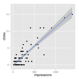
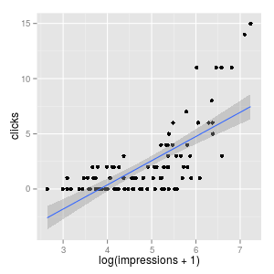
One issue about the linear regression model is that, most of the data points are concentrated, with click # < 5. And there are a few points that are highly distant from this cluster. This is not a good pattern for regression, because shifting those distant points a little would make our estimate change a lot. By taking the logarithm transform, those distant points are pulled close to the majority of data points, and our regression estimate would be more stable.
Again, the caveat here is how to interpret your estimate in practice. Taking the logarithm means that as impression number increases, the click-through number increases, but they do not increase linearly. The click-through increase as impression # increase from 0-100 is much larger than the click-through increase as impression # increase from 1000-1100.
Does it make sense? A plausible interpretation is that, as you increase your impression #, part of that will be directed to the existing audience. In other words, you are introducing fewer new audience. The first 100 impressions all go to people who have never watched your ad; the 1000-100 impression may include 50 people that have already watched your ad, and those people are not going to click your display.
This interpretation may sound intriguing, but it is ad-hoc. As George Box’s famous cliche, “all models are wrong, but some are useful.” Perhaps the best way to justify your model is to look at the data, and it is the data where the story lies in.