Chandler Zuo

Logistic Regression with Imbalanced Data

25 Mar 2015 | Chandler

Logistic regression is a useful model in predicting binary events and has lots of applications. In real life lots of applications target the prediction for risk events. For example, insurance companies need predict the probability of an adverse event, credit companies need predict the credit fraud event. In these cases, the response variable is the binary indicator for the risk event, i.e. 1 if the risk event occurs. The logistic regression model uses a class of predictors to build a function that stand for the probability for such risk event.

A typical problem for these applications is that, the risk event is quite rare in practice. For example, your data may contain 10,000 observations, but only 5% of them have risk events. If we call the observations with response 1 as the positive set, and the rest as the negative set, majority of the observations are from the negative set. The positive and negative sets are extremely imbalanced. A consequence is that, when validating your fit using test data set, only a small proportion in the positive set can be correctly identified.

Is there a remedy for this problem? There are two commonly discussed methods, both try to balance the data. The first method is to subsample the negative set to reduce it to be the same size as the positive set, then fit the logistic regression model with the reduced data set. The second method is to use weighted logistic regression. For a data set containing 5% positives and 95% negatives, we can assign each positive observation a weight of 0.95, and each negative observation a weight of 0.05.

As an example, I generate a training data set of 10,000 observations, with about 10% positives. I also generate a testing data set with the same model and the same structure. For this testing data set, it contains 1024 positives. Using the naive logistic regression, it correctly identifies 21 among them as positives. Using subsampled training data, or the weighted logistic regression, this number becomes 769 or 766 immediately.

Is this a nice result? A simple fix for a seemingly complicated problem, isn’t it? Life experience tells us that no lunch is free. If a simple modification makes such a drastic improvement, some price must be paid. What is it?

Well, let’s step back a little. There are two categories in the data set: positive and negative. We have only looked at the predicting error in the positive set. How about the negative set? To that end, I generate the confusion matrices for each of the three logistic regression methods. Each confusion matrix is a two by two matrix, with the rows corresponding to the true category, and the columns representing the predicted category. The confusion matrix for the naive logistic regression is:

	Predicted
True	NEG	POS
NEG	8976	0
POS	1003	21

In this case, among the 8976 true negatives, all of them are predicted as negatives. Among the 1024 true positives, 21 of them are predicted as positives, and the rest are predicted as negatives. Although we are making lousy prediction on the positive set, we can predict the negative set perfectly.

How about the other cases?

Subsampled:

	Predicted
True	NEG	POS
NEG	6778	2198
POS	255	769

Weighted Logistic Regression:

	Predicted
True	NEG	POS
NEG	6785	2191
POS	258	766

We see that both of them predict a fair amount of true negatives as positives, the so called Type-I error. This is the price we pay!

So if we want to combine the error rates on both categories, how should we compare the three methods? One answer is the ROC curve. To generate such a curve, first we need to realize that logistic regression models only output the predicted probability values for each observation. To convert such probabilities to actual predictions we need to set a cut-off. For the previous confusion matrices, we have used the cut-off as 0.5, and assigned observations with probabilities >=0.5 as the predicted positives. This is the usual choice in practice. Within each confusion matrix, we can compute two quantities:

False Positive Rate (FPR) = (# True negatives which are predicted as positives) / (# True negatives);

True Positive Rate (TPR, or Power) = (# True positives which are predicted as Positives) / (# True positives).

As we vary this cut-off, we can get a series of confusion matrices, and correspondingly a series of (FPR, TPR) pairs. Plotting these points gives the ROC curve.

So here are the ROC curves of our data:

Proportion of Positives = 10%:

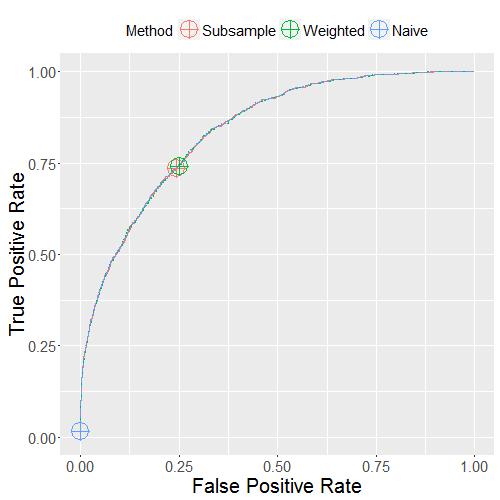
Here, I also mark the point with the probability cut-off 0.5 by the crossed circles. We see that the ROC curves of the three methods are quite close! The only difference is that at the cut-off 0.5, the naive logistic regression differs from the other two. It is much more conservative: much lower power but also much lower FPR. However, we can also pick higher cut-offs with the subsampled or the weighted logistic regression model, and achieve the same conservative result. Alternatively, if we pick lower cut-off for the naive logistic regression model, it can achieve the same result as the subsampled or the weighted logistic regression. If we pick the cut-off for each method to control the FPR at the same level, then none of the methods would have higher power than others. In that sense, no method is better than another.

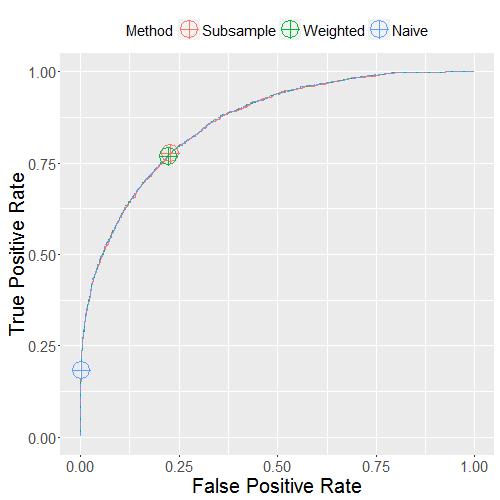
We can get the ROC curves with data of different proportion of positives:

Proportion of Positives = 13%. We can see similar patterns as the previous figure:

Proportion of Positives = 50%. In this last case, the three marked points overlap because the data is balanced between the two categories:

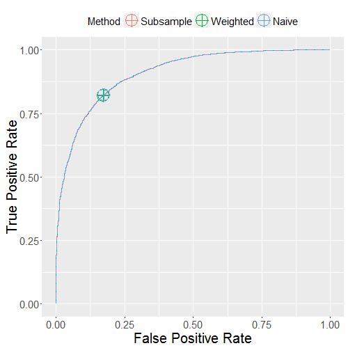
The conclusion is that, neither subsampling training data nor weighted logistic regression gives a better model than the naive method. The three methods differ only by how they select a cut-off to convert the fitted probability values to the positive / negative labels.

So next time, if you feel your positive set is not fitted well, lower the cut-off and see what happens.

Here are the codes.