Integrating ROC Curves, Model Ensembling and IDR
PROBLEM
In the previous post, I proposed an method for pooling multiple ranked lists from different model-based probability estimation. The method was applicable when we have a binary classification task for a certain data set, with it being partitioned into multiple subsets, and different classification models built for each subset. Usually, this happens when we assume some clustering structure among observations in the original data set, and decide that it is the best to fit different classification models within each cluster - an idea analogous to the concept of mixture modeling.
In this post, I would like to discuss another related problem on pooling binary classification models. When we have multiple classification models for the same data set, each of which produce a different probabilistic ranking of all observations in the data set, how should we pool model results in order to get the optimal ranking of all observations? Notice that in this case, we do not partition the data set into subsets; each model is applied to the entire data set. As a result, for each observation, we have multiple estimation from different models, and we would like to combine all the different estimates together in order to produce some score that can provide the best ranking among observations.
This problem is closely linked to the concept of Ensemble Modeling, or Ensemble Learning, a very common strategy used in predictive modeling. The idea is that, when we have different algorithms used for the same classification task, rather than picking one “dictator” algorithm and disregard all the other algorithms, it is better to run a “poll” on the results of all different algorithms and produce a “democratic” result. This hopefully can reduce the prediction variability of using one single algorithm. In practice, ensembling methods are vastly useful. If you have Kaggle competition experience, you must be conviced of this strategy.
A key challenge, therefore, on model ensembling is to identify the best pooling strategy. Averaging prediction from different models is probably the most common choice, but is there any better way to do so? As a naive example, consider two observations A and B, and we build two binary classification models for them. Probability estimation for A under the two models is 0.1 and 0.9, while probability estimation for B is 0.4 and 0.6. The average probability estimation for A and B is both 0.5, but estimation for A has more variation. It is a tough decision to say which one is more likely to have Class 1 or Class 0.
SOLUTION
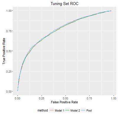
I illustrate the solution using an example, where I fitted the UCI Credit Default Dataset using two gradient boosting models. The codes of this example are available here. After splitting the data set into training, tuning and testing sets, I fitted two gradient boosting models on the training set, and produced the ROC curve based on each model for the tuning set as the following.
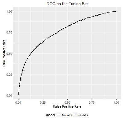
ROC curves show the relationship between False Positive Rate and True Positive Rate within each model. They can be visualized in another way: how either FPR or TPR varies according to the probability estimates of a model, as I show below:
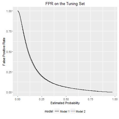
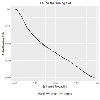
Rather than presenting the two curves separately in a 2-D space, now I reconsider the TPR and FPR as the outcomes of bivariate functions. Each bivariate function uses the probability estimates from the two models, and maps to the TPR/FPR value. In this way, the TPR and FPR can be visualized in the following plots:
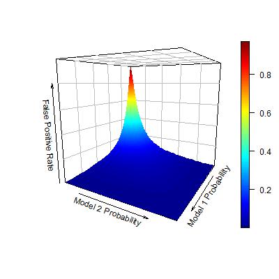
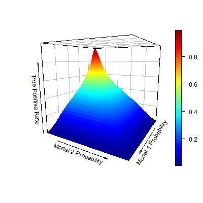
Now, consider the objective of seeking an ordering of observations that maximize the AUC. Following the logic in my previous post, this problem is identical to: given each level of FPR, find a set of observations to be predicted as positive, so that the TPR is maximized. Now that I have seen both TPR and FPR as bivariate functions of individual model probability estimates, this problem seems quite obvious to solve. Given each level of FPR, we can identify an area for the pair of two model probability estimates such that FPR is controlled under this level. Within this area, I can further find the pair of model probability estimates such that TPR is maximized.
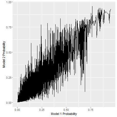
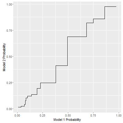
There is one problem for this seemingly obvious solution. Given a fixed level of FPR, the above approach yields the optimal pair of probability thresholds for both models. The maximum TPR is achieved if all observations that satisfy both thresholds are estimated as positive. However, as we increase the FPR values, the sets of observations estimated as positive under this rule are not partially ordered. In other words, suppose we have two FPR thresholds, FPR1 < FPR2, estimated positive observations under FPR1 should be a subset of those under FPR2, but there is no control for this. One reflection of this phenomena is that, when we plot the path of the pair of probability thresholds as the FPR level varies, the path is quite noisy as below. If the partial ordering relationship holds, however, this path should be monotone non-dedecreasing.
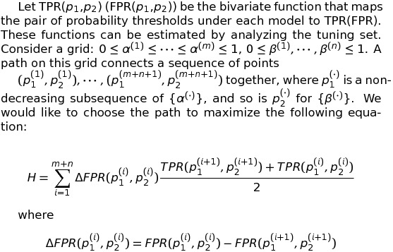
Therefore, the real underlying problem is: how to find a sequence of pairs of probability thresholds for the two models, where either threshold is a monotone non-decreasing function of the other, such that TPR and FPR under such a sequence of thresholds will achieve the maximum AUC value.
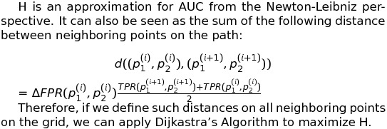
At first, this problem may seem too difficult to be solved. Luckily, I found that this problem can be translated to an path searching problem solved by Dijkastra’s Algorithm. The translation can be outlined as the following.
Implementation of this algorithm is a bit tricky for R, since it involves iterative non-vector calculation. As I used the Rcpp package to implement it, I achieved the following path for this example:
This path now entails a third ROC curve. As I plot it together with the ROC curves from individual models, I can see that the third curve is better than individual ones, which is totally expected.
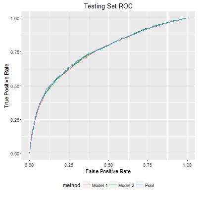
Finally, we can map each pair of probability estimates for observations in the testing set to the path, and create an ordered list for testing set observations. The ROC plot shows that my approach does improve individual model estimates. In the following figure, AUC for Model 1 and Model 2 are 0.7474 and 0.7501, while the pooled prediction has AUC of 0.7514. Although the improvement was marginal, as I repeated the experiment, I did see that the improvement is consistently reproducible. This could be very significant in practice.
DISCUSSION
Another possible approach to solve this problem is by using Irreproducible Discovery Rate(IDR), a method proposed by Peter Bickel’s team. Interestingly, this method was not proposed from the machine learning context, but from the context of the peak calling problem, the problem to identify protein binding regions on the genome. Protein binding status on the genome are binary, and in order to identify binding regions, multiple experiments are repeated under the same protocol to reduce the chance of idiosyncratic discoveries. When applying the same algorithm to different data sets, the classification probability estimates are different, and IDR offers a way to integrate the estimates from different experimental data to get a more robust estimate. IDR was developed to pool results from the same algorithm of different data sets, while model ensembling deals with pooling results from different algorithms on the same data set. However, the fundamental problem underlying these two is the same: pooling multiple estimation results on the same set of observations.
There is one key difference between IDR and my proposed approach in this post. IDR does not utilize the ROC curve from individual models, because for peak calling data sets the observations are not labeled, and IDR can only rely on p-values from hypotheses testing. As a result, IDR relies on parametric mixture models, with a separate task to estimate the class labels in the training set. This is a more challenging problem than the case considered in this post, where we already have labeled training set and can directly start from the empirical distribution of probability estimates within each class. Therefore, my conjecture is that for classification problems, my approach works better because it utilizes more information.
The example in the post shows how to optimally integrate results from two models. When multiple models are available, the approach described in the post can be readily extended, although actual implementation to calculate the TPR/FPR as multi-variate function of individual model estimates can be quite intensive, and so is for Dijkastra’s algorithm. This approach can even be adopted for ensembling lower level models, for example, to optimize the weights of individual decision trees within a single gradient boosting model.
(c)2016-2025 CHANDLER ZUO ALL RIGHTS PRESERVED