A PyTorch Example to Use RNN for Financial Prediction
While deep learning has successfully driven fundamental progress in natural language processing and image processing, one pertaining question is whether the technique will equally be successful to beat other models in the classical statistics and machine learning areas to yield the new state-of-the-art methodology for uncovering the underlying data patterns. One such area is the prediction of financial time series, a notoriously difficult problem given the fickleness of such data movement. In this blog, I implement one recently proposed model for this problem. For myself, this is more of a learning process to implement the deep learning technology for real data, which I would like to share my experience with others.
The Model
The model I have implemented is proposed by the paper A Dual-Stage Attention-Based Recurrent Neural Network for Time Series Prediction. The Dual-Stage Attention-Based RNN (a.k.a. DA-RNN) model belongs to the general class of Nonlinear Autoregressive Exogenous (NARX) models, which predict the current value of a time series based on historical values of this series plus the historical values of multiple exogenous time series. A linear counterpart of a NARX model is the ARMA model with exogenous factors.
There are two important concepts in the DA-RNN model. The first one is the popular Recursive Neural Network model, which has enjoyed big success in the NLP area. On a high level, RNN models are powerful to exhibit quite sophisticated dynamic temporal structure for sequential data. RNN models come in many forms, one of which is the Long-Short Term Memory(LSTM) model that is widely applied in language models. The second concept is the Attention Mechanism. Attention mechanism somewhat performs feature selection in a dynamic way, so that the model can keep only the most useful information at each temporal stage. Many successful deep learning models nowadays combine attention mechanism with RNN, with examples including machine translation.
The DA-RNN model, on the high level, includes two LSTM networks with attention mechanism. The first LSTM network encodes information among historical exogenous data, and its attention mechanism performs feature selection to select the most important exogenous factors. Based on the output of the first LSTM network, the second LSTM network further combines the information from exogenous data with the historical target time series. The attention mechanism in the second network performs feature selection in the time domain, i.e., it applies weights to information at different historical time points. The final prediction, therefore, is based on feature selection in both the dimension of exogenous factors and time. Unlike classical feature selection in statistical models, DA-RNN selects features dynamically. In other words, the weights on factors and time points are changing across time. One inaccurate analogy, perhaps, is a regression model with ARMA errors, with time-varying coefficients for both the exogenous factors and the ARMA terms.
PyTorch
My experiment is implemented in PyTorch. Why PyTorch? From my experience, it has better integration with Python as compared to some popular alternatives including TensorFlow and Keras. It also seems the only package I have found so far that enables interchanging between auto-grad calculations and other calculations. This gives great flexibility for me as a person with primarily model building and not engineering backgrounds:
- PyTorch codes are easy to debug by inserting python codes to peep into intermediate values between individual auto-grad steps;
- PyTorch also enables experimenting ideas by adding some calculations between different auto-grad steps. For example, it is easy to implement an algorithm that iterates between discrete calculations and auto-grad calculations.
A PyTorch tutorial for machine translation model can be seen at this link. My implementation is based on this tutorial.
Data
I use the NASDAQ 100 Stock Data as mentioned in the DA-RNN paper. Unlike the experiment presented in the paper, which uses the contemporary values of exogenous factors to predict the target variable, I exclude them. For this data set, the exogenous factors are individual stock prices, and the target time series is the NASDAQ stock index. Using the current prices of individual stocks to predict the current NASDAQ index is not really meaningful, thus I have made this change.
Codes
My main notebook is shown below. Supportive codes can be found here.
First, I declare the Python module dependencies.
import torch
from torch import nn
from torch.autograd import Variable
from torch import optim
import torch.nn.functional as F

import matplotlib
# matplotlib.use('Agg')
%matplotlib inline

import datetime as dt, itertools, pandas as pd, matplotlib.pyplot as plt, numpy as np

import utility as util

global logger

util.setup_log()
util.setup_path()
logger = util.logger
text_process.logger = logger

use_cuda = torch.cuda.is_available()
logger.info("Is CUDA available? %s.", use_cuda)
Second, I build the two Attention-Based LSTM networks, named by encoder and decoder respectively. For easier understanding I annotate my codes with equation numbers in the DA-RNN paper.
class encoder(nn.Module):
    def __init__(self, input_size, hidden_size, T, logger):
        # input size: number of underlying factors (81)
        # T: number of time steps (10)
        # hidden_size: dimension of the hidden state
        super(encoder, self).__init__()
        self.input_size = input_size
        self.hidden_size = hidden_size
        self.T = T

        self.logger = logger

        self.lstm_layer = nn.LSTM(input_size = input_size, hidden_size = hidden_size, num_layers = 1)
        self.attn_linear = nn.Linear(in_features = 2 * hidden_size + T - 1, out_features = 1)

    def forward(self, input_data):
        # input_data: batch_size * T - 1 * input_size
        input_weighted = Variable(input_data.data.new(input_data.size(0), self.T - 1, self.input_size).zero_())
        input_encoded = Variable(input_data.data.new(input_data.size(0), self.T - 1, self.hidden_size).zero_())
        # hidden, cell: initial states with dimention hidden_size
        hidden = self.init_hidden(input_data) # 1 * batch_size * hidden_size
        cell = self.init_hidden(input_data)
        # hidden.requires_grad = False
        # cell.requires_grad = False
        for t in range(self.T - 1):
            # Eqn. 8: concatenate the hidden states with each predictor
            x = torch.cat((hidden.repeat(self.input_size, 1, 1).permute(1, 0, 2),
                           cell.repeat(self.input_size, 1, 1).permute(1, 0, 2),
                           input_data.permute(0, 2, 1)), dim = 2) # batch_size * input_size * (2*hidden_size + T - 1)
            # Eqn. 9: Get attention weights
            x = self.attn_linear(x.view(-1, self.hidden_size * 2 + self.T - 1)) # (batch_size * input_size) * 1
            attn_weights = F.softmax(x.view(-1, self.input_size)) # batch_size * input_size, attn weights with values sum up to 1.
            # Eqn. 10: LSTM
            weighted_input = torch.mul(attn_weights, input_data[:, t, :]) # batch_size * input_size
            # Fix the warning about non-contiguous memory
            # see https://discuss.pytorch.org/t/dataparallel-issue-with-flatten-parameter/8282
            self.lstm_layer.flatten_parameters()
            _, lstm_states = self.lstm_layer(weighted_input.unsqueeze(0), (hidden, cell))
            hidden = lstm_states[0]
            cell = lstm_states[1]
            # Save output
            input_weighted[:, t, :] = weighted_input
            input_encoded[:, t, :] = hidden
        return input_weighted, input_encoded

    def init_hidden(self, x):
        # No matter whether CUDA is used, the returned variable will have the same type as x.
        return Variable(x.data.new(1, x.size(0), self.hidden_size).zero_()) # dimension 0 is the batch dimension

class decoder(nn.Module):
    def __init__(self, encoder_hidden_size, decoder_hidden_size, T, logger):
        super(decoder, self).__init__()

        self.T = T
        self.encoder_hidden_size = encoder_hidden_size
        self.decoder_hidden_size = decoder_hidden_size

        self.logger = logger

        self.attn_layer = nn.Sequential(nn.Linear(2 * decoder_hidden_size + encoder_hidden_size, encoder_hidden_size),
                                         nn.Tanh(), nn.Linear(encoder_hidden_size, 1))
        self.lstm_layer = nn.LSTM(input_size = 1, hidden_size = decoder_hidden_size)
        self.fc = nn.Linear(encoder_hidden_size + 1, 1)
        self.fc_final = nn.Linear(decoder_hidden_size + encoder_hidden_size, 1)

        self.fc.weight.data.normal_()

    def forward(self, input_encoded, y_history):
        # input_encoded: batch_size * T - 1 * encoder_hidden_size
        # y_history: batch_size * (T-1)
        # Initialize hidden and cell, 1 * batch_size * decoder_hidden_size
        hidden = self.init_hidden(input_encoded)
        cell = self.init_hidden(input_encoded)
        # hidden.requires_grad = False
        # cell.requires_grad = False
        for t in range(self.T - 1):
            # Eqn. 12-13: compute attention weights
            ## batch_size * T * (2*decoder_hidden_size + encoder_hidden_size)
            x = torch.cat((hidden.repeat(self.T - 1, 1, 1).permute(1, 0, 2),
                           cell.repeat(self.T - 1, 1, 1).permute(1, 0, 2), input_encoded), dim = 2)
            x = F.softmax(self.attn_layer(x.view(-1, 2 * self.decoder_hidden_size + self.encoder_hidden_size
                                                )).view(-1, self.T - 1)) # batch_size * T - 1, row sum up to 1
            # Eqn. 14: compute context vector
            context = torch.bmm(x.unsqueeze(1), input_encoded)[:, 0, :] # batch_size * encoder_hidden_size
            if t < self.T - 1:
                # Eqn. 15
                y_tilde = self.fc(torch.cat((context, y_history[:, t].unsqueeze(1)), dim = 1)) # batch_size * 1
                # Eqn. 16: LSTM
                self.lstm_layer.flatten_parameters()
                _, lstm_output = self.lstm_layer(y_tilde.unsqueeze(0), (hidden, cell))
                hidden = lstm_output[0] # 1 * batch_size * decoder_hidden_size
                cell = lstm_output[1] # 1 * batch_size * decoder_hidden_size
        # Eqn. 22: final output
        y_pred = self.fc_final(torch.cat((hidden[0], context), dim = 1))
        # self.logger.info("hidden %s context %s y_pred: %s", hidden[0][0][:10], context[0][:10], y_pred[:10])
        return y_pred

    def init_hidden(self, x):
        return Variable(x.data.new(1, x.size(0), self.decoder_hidden_size).zero_())
The next code chunk implements an object for all steps in the modeling pipeline.
# Train the model
class da_rnn:
    def __init__(self, file_data, logger, encoder_hidden_size = 64, decoder_hidden_size = 64, T = 10,
                 learning_rate = 0.01, batch_size = 128, parallel = True, debug = False):
        self.T = T
        dat = pd.read_csv(file_data, nrows = 100 if debug else None)
        self.logger = logger
        self.logger.info("Shape of data: %s.\nMissing in data: %s.", dat.shape, dat.isnull().sum().sum())

        self.X = dat.loc[:, [x for x in dat.columns.tolist() if x != 'NDX']].as_matrix()
        self.y = np.array(dat.NDX)
        self.batch_size = batch_size

        self.encoder = encoder(input_size = self.X.shape[1], hidden_size = encoder_hidden_size, T = T,
                              logger = logger).cuda()
        self.decoder = decoder(encoder_hidden_size = encoder_hidden_size,
                               decoder_hidden_size = decoder_hidden_size,
                               T = T, logger = logger).cuda()

        if parallel:
            self.encoder = nn.DataParallel(self.encoder)
            self.decoder = nn.DataParallel(self.decoder)

        self.encoder_optimizer = optim.Adam(params = itertools.ifilter(lambda p: p.requires_grad, self.encoder.parameters()),
                                           lr = learning_rate)
        self.decoder_optimizer = optim.Adam(params = itertools.ifilter(lambda p: p.requires_grad, self.decoder.parameters()),
                                           lr = learning_rate)
        # self.learning_rate = learning_rate

        self.train_size = int(self.X.shape[0] * 0.7)
        self.y = self.y - np.mean(self.y[:self.train_size]) # Question: why Adam requires data to be normalized?
        self.logger.info("Training size: %d.", self.train_size)

    def train(self, n_epochs = 10):
        iter_per_epoch = int(np.ceil(self.train_size * 1. / self.batch_size))
        logger.info("Iterations per epoch: %3.3f ~ %d.", self.train_size * 1. / self.batch_size, iter_per_epoch)
        self.iter_losses = np.zeros(n_epochs * iter_per_epoch)
        self.epoch_losses = np.zeros(n_epochs)

        self.loss_func = nn.MSELoss()

        n_iter = 0

        learning_rate = 1.

        for i in range(n_epochs):
            perm_idx = np.random.permutation(self.train_size - self.T)
            j = 0
            while j < self.train_size:
                batch_idx = perm_idx[j:(j + self.batch_size)]
                X = np.zeros((len(batch_idx), self.T - 1, self.X.shape[1]))
                y_history = np.zeros((len(batch_idx), self.T - 1))
                y_target = self.y[batch_idx + self.T]

                for k in range(len(batch_idx)):
                    X[k, :, :] = self.X[batch_idx[k] : (batch_idx[k] + self.T - 1), :]
                    y_history[k, :] = self.y[batch_idx[k] : (batch_idx[k] + self.T - 1)]

                loss = self.train_iteration(X, y_history, y_target)
                self.iter_losses[i * iter_per_epoch + j / self.batch_size] = loss
                #if (j / self.batch_size) % 50 == 0:
                #    self.logger.info("Epoch %d, Batch %d: loss = %3.3f.", i, j / self.batch_size, loss)
                j += self.batch_size
                n_iter += 1

                if n_iter % 10000 == 0 and n_iter > 0:
                    for param_group in self.encoder_optimizer.param_groups:
                        param_group['lr'] = param_group['lr'] * 0.9
                    for param_group in self.decoder_optimizer.param_groups:
                        param_group['lr'] = param_group['lr'] * 0.9

            self.epoch_losses[i] = np.mean(self.iter_losses[range(i * iter_per_epoch, (i + 1) * iter_per_epoch)])
            if i % 10 == 0:
                self.logger.info("Epoch %d, loss: %3.3f.", i, self.epoch_losses[i])

            if i % 10 == 0:
                y_train_pred = self.predict(on_train = True)
                y_test_pred = self.predict(on_train = False)
                y_pred = np.concatenate((y_train_pred, y_test_pred))
                plt.figure()
                plt.plot(range(1, 1 + len(self.y)), self.y, label = "True")
                plt.plot(range(self.T , len(y_train_pred) + self.T), y_train_pred, label = 'Predicted - Train')
                plt.plot(range(self.T + len(y_train_pred) , len(self.y) + 1), y_test_pred, label = 'Predicted - Test')
                plt.legend(loc = 'upper left')
                plt.show()

    def train_iteration(self, X, y_history, y_target):
        self.encoder_optimizer.zero_grad()
        self.decoder_optimizer.zero_grad()

        input_weighted, input_encoded = self.encoder(Variable(torch.from_numpy(X).type(torch.FloatTensor).cuda()))
        y_pred = self.decoder(input_encoded, Variable(torch.from_numpy(y_history).type(torch.FloatTensor).cuda()))

        y_true = Variable(torch.from_numpy(y_target).type(torch.FloatTensor).cuda())
        loss = self.loss_func(y_pred, y_true)
        loss.backward()

        self.encoder_optimizer.step()
        self.decoder_optimizer.step()

        return loss.data[0]

    def predict(self, on_train = False):
        if on_train:
            y_pred = np.zeros(self.train_size - self.T + 1)
        else:
            y_pred = np.zeros(self.X.shape[0] - self.train_size)

        i = 0
        while i < len(y_pred):
            batch_idx = np.array(range(len(y_pred)))[i : (i + self.batch_size)]
            X = np.zeros((len(batch_idx), self.T - 1, self.X.shape[1]))
            y_history = np.zeros((len(batch_idx), self.T - 1))
            for j in range(len(batch_idx)):
                if on_train:
                    X[j, :, :] = self.X[range(batch_idx[j], batch_idx[j] + self.T - 1), :]
                    y_history[j, :] = self.y[range(batch_idx[j],  batch_idx[j]+ self.T - 1)]
                else:
                    X[j, :, :] = self.X[range(batch_idx[j] + self.train_size - self.T, batch_idx[j] + self.train_size - 1), :]
                    y_history[j, :] = self.y[range(batch_idx[j] + self.train_size - self.T,  batch_idx[j]+ self.train_size - 1)]

            y_history = Variable(torch.from_numpy(y_history).type(torch.FloatTensor).cuda())
            _, input_encoded = self.encoder(Variable(torch.from_numpy(X).type(torch.FloatTensor).cuda()))
            y_pred[i:(i + self.batch_size)] = self.decoder(input_encoded, y_history).cpu().data.numpy()[:, 0]
            i += self.batch_size
        return y_pred
The actual execution of the algorithm can be triggered as the following:
io_dir = '~/nasdaq'

model = da_rnn(file_data = '{}/data/nasdaq100_padding.csv'.format(io_dir), logger = logger, parallel = False,
              learning_rate = .001)

model.train(n_epochs = 500)

y_pred = model.predict()

plt.figure()
plt.semilogy(range(len(model.iter_losses)), model.iter_losses)
plt.show()

plt.figure()
plt.semilogy(range(len(model.epoch_losses)), model.epoch_losses)
plt.show()

plt.figure()
plt.plot(y_pred, label = 'Predicted')
plt.plot(model.y[model.train_size:], label = "True")
plt.legend(loc = 'upper left')
plt.show()
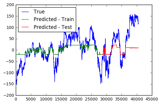
Results can be presented in the following figures. Notice that the target time series are normalized to have mean 0 within the training set; otherwise the network is extremely slow to converge.
Model Fit after 10 Epochs
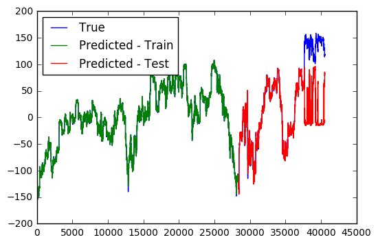
Model Fit after 500 Epochs
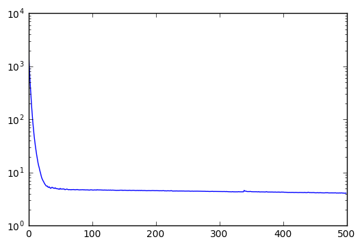
Training Loss across 500 Epochs
From the first two figures, it is interesting to see that how the model gradually expands its range of prediction across training epochs. Eventually, the model can predict quite accurately within the whole range of the training data, but fails to predict outside this regime. Regime shifts in the stock market, apparently, remains an unpredictable beast.
Updates 10/1/2018
Thanks to Sean Aubin’s contribution, an updated version of these codes is now available. These codes are written in Python3 and depend on more recent versions of PyTorch. The updated codes also use functional programming that may suit some people’s flavor. Please refer to his repository and applaud for his work!
(c)2017-2026 CHANDLER ZUO ALL RIGHTS PRESERVED