Regularization Effect of Adversarial Examples Learning
ADVERSARIAL EXAMPLES
Neural network models can be susceptible to adversarial examples, which are perturbed input data too small to be detected by human yet tricky enough to confuse a trained model into making errors. The following is a famous example from Goodfellow et al. 2014. While the left photo is categorized correctly in the panda category, with some specifically constructed noises, the right photo is incorrectly categorized as in the gibbon category. In fact, such noises can be constructed to confuse the network in an arbitrary way. Daniel Geng and Rishi Veerapaneni’s blog illustrates how to do so using image classification as an example.

The key step of constructing adversarial examples is to find the direction of the input noise that the network is sensitive to. A neural network input often comes in high dimensions. For an RGB image with 128x128px, the dimension is 128x128x3=49152. With such high dimensions, it is unrealistic to assume a neural network model to be robust against noises in all dimensions. To find the most malicious direction of the input noise is essentially to find the dimensions in the input data which a neural network is most sensitive to. Mathematically, such malicious directions can be found by calculating the derivative of the objective function the trained model minimizes against the input data. The derivative calculation is the right tool to find malicious directions because by definition, it is used to find how a function’s input can be minimally perturbed to bring the maximally change in its output.
FAST GRADIENT SIGN METHOD AND LASSO
We know that neural network models are sensitive to adversarial examples. How can we make neural network to be robust against adversarial noises? Since we already know how to generate such adversarial noises, we can simply augment the training data using these adversarial examples. This idea was proposed by Goodfellow et al. 2014. Specifically, they proposed the Fast Gradient Sign Method (FGSM). This method generates noises that has the same scale in every dimension, but the sign in each dimension is determined by the gradient calculation. The mathematical formula for an adversarial example is:
![]()
In a 1-layer neural network model with sigmoid activation, Goodfellow et al. 2014 reckons that such learning is closely related to LASSO penalty. This is because the objective function with FGSM examples is:
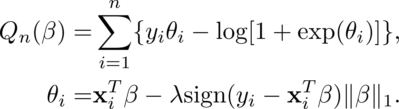
Comparing this to the objective function of LASSO-penalized likehood estimation:
![]()
FGSM simply changes the order between sigmoid activation and imposing the LASSO penalty. Because of this, Goodfellow et al. 2014 states that FGSM has regularization effect similar to LASSO. The difference between these two types of regularization is that the penalty in FGSM automatically deactivates if the prediction is confident enough, while LASSO penalty focuses more on the worst case scenarios.
GENERALIZED FGSM
The relationship between FGSM and LASSO motivates me to study the asymptotic behavior of FGSM in simple regression models. In fact, despite much numerical results showing the benefit of using FGSM for real data, there is not much theoretical justification. For LASSO, decades of theoretical research have yielded much understanding on its benefits, which have well explained its role in neural network regularization (commonly known as L1 weight decay). If we can derive statistical properties for FGSM in simple regression models, such as linear regression and logistic regression, the insights may help us interpret its effectiveness in deep neural network models.
My recent paper is an effort in this direction. The theoretical framework is built for Generalized FGSM estimation for generalized linear models (GLM). The theory is built for estimation with the following objective function:
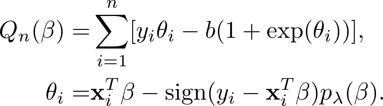
This setting is more general than FGSM with sigmoid activation in that
- the activation function can not only be the sigmoid function;
- the penalty function can not only be LASSO.
The first point is actually a limit; the framework includes linear regression and logistic regression, but exclude activation functions such as ReLU that does not correspond to GLMs. The second point is, however, more interesting. Before, we have seen that if the penalty function is LASSO, the objective function corresponds to learning using FGSM adversarial examples. If we choose another penalty function, such as general Lr shrinkage or [SCAD] penalty, the corresponding schema to generate adversarial noises is:
![]()
This gives a large number of ways to generate adversarial examples, which can be interesting to evaluate empirically.
ASYMPTOTICS FOR FGSM-TYPE LEARNING
It is already know that penalized likelihood estimation for GLM has three properties:
- Root-n consistency. In layman’s term, the standard error for the parameter estimator is halved every time the training sample is quadrupled. This is a desirable statistical property for regression models, and is the best rate achievable because of Cramer-Rao’s Bound.
- Sparsity. The parameter estimator is sparse. This creates some bias but may reduce the overall estimation error due to bias-variance tradeoff.
- Oracle property for non-concave penalties. If the true parameter is sparse, the estimated parameter is almost as accurate as if we knew which parameters were zero. This only happens if the penalty function is non-concave, such as SCAD or Lr with 0<r<1.
The main result of My paper is that all these properties are inherited by Generalized FGSM. Moreover, the asymptotic distribution is highly similar to penalized likelihood estimation. For both methods, the asymptotic distribution follows the form
![]()
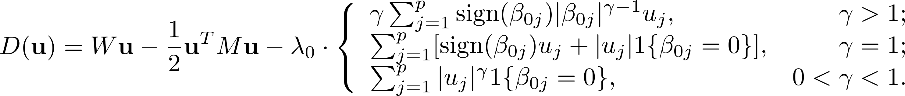
For Generalized FGSM, the asymptotically maximized function with Lr penalty is:

For penalized likelihood estimation, the corresponding asymptotically maximized function is:
COMPARING GENERALIZED FGSM WITH PENALIZED LIKELIHOOD
The asymptotic results have two implications.
Automatically Scaled Penalty
The multipler of the penalty in Generalized FGSM is automatically scaled by the dispersion of error. This is desirable since the tuning parameter, lambda, can be uncoupled from noise level in the data, and thus be selected based on the sparsity level alone. For penalized likelihood estimation, on the other hand, the selected lambda need be scaled against a heuristically estimated noise level.
Sign Neutrality
Generalized FGSM is different from penalized likelihood estimation if the training data is not sign neutral. This concept is related to the quantity V in the asymptotic equations:
![]()
When V is non-zero, it introduces additional bias compared to penalized likelihood estimation. For linear regression models, V=0 requires trivial conditions that can be assumed true in most practical cases. However, for logistic regression, V=0 requires that the data sampling need be balanced in a certain way.
Sign neutrality requires that the average sign of errors across all training data is roughly 0. To see how balanced the sampling should be in a logistic regression model, consider a single binary random variable Y with probability p for Y=1 and 1-p for Y=0. The expected sign of the error Y-p is 1p+(-1)(1-p)=2p-1. This is equal to 0 only when p=0.5. Intuitively, if the training data sampling is sign neutral, the average binary probability across all observations should be roughly 0.5. This condition is not satisfied for any data that are not balanced between the two categories.
One thing to mention here is that, such additional bias does not necessarily make Generalized FGSM inferior to penalized likelihood. Just as LASSO penalty, biases in estimation can trade off with variance to improve overall estimation accuracy. Whether the additional bias in Generalized FGSM improves such tradeoff requires future analysis.
CONCLUSIONS
Asymptotics is an important topic in theoretical statistics. Yet, I have often heard critism for such research in that such theory yields little practical usage. As an applied researcher myself, however, I do feel such critism is unfair. Methodological research sometimes move much faster than mathematical theory. But it is not wise to undermine the value of such theory. At least, such theory help answer three questions: why certain methodology works, how it can be generalized, and where its boundary is.
There is no doubt that FGSM and the general adversarial examples learning is highly successful. With so much empirical success, I have been curious of the its underlying mathematical mechanism. Such curiosity motivates me to develop the theory in this paper. Of course, my theory is far from comprehensive, but it does shed light on to the three questions mentioned above. Root-n consistency, sparsity, and oracle properties are all nice properties that explains its success; its generalization can be induced by a large number of penalty functions already used in penalized likelihood; one of its boundaries may be sign neutrality. The theory so far is entirely based on 1-layer neural network models, but I hypothesize such properties have strong implications for deep neural network models as well.
(c)2017-2026 CHANDLER ZUO ALL RIGHTS PRESERVED